options(repr.plot.width = 12, repr.plot.height = 6)Ch08 ARIMA 모형의 적합
EX 8.6 가스공급비율
z <- scan("gas.txt", what=list(0,0))head(z)-
- -0.109
- 0
- 0.178
- 0.339
- 0.373
- 0.441
- 0.461
- 0.348
- 0.127
- -0.18
- -0.588
- -1.055
- -1.421
- -1.52
- -1.302
- -0.814
- -0.475
- -0.193
- 0.088
- 0.435
- 0.771
- 0.866
- 0.875
- 0.891
- 0.987
- 1.263
- 1.775
- 1.976
- 1.934
- 1.866
- 1.832
- 1.767
- 1.608
- 1.265
- 0.79
- 0.36
- 0.115
- 0.088
- 0.331
- 0.645
- 0.96
- 1.409
- 2.67
- 2.834
- 2.812
- 2.483
- 1.929
- 1.485
- 1.214
- 1.239
- 1.608
- 1.905
- 2.023
- 1.815
- 0.535
- 0.122
- 0.009
- 0.164
- 0.671
- 1.019
- 1.146
- 1.155
- 1.112
- 1.121
- 1.223
- 1.257
- 1.157
- 0.913
- 0.62
- 0.255
- -0.28
- -1.08
- -1.551
- -1.799
- -1.825
- -1.456
- -0.944
- -0.57
- -0.431
- -0.577
- -0.96
- -1.616
- -1.875
- -1.891
- -1.746
- -1.474
- -1.201
- -0.927
- -0.524
- 0.04
- 0.788
- 0.943
- 0.93
- 1.006
- 1.137
- 1.198
- 1.054
- 0.595
- -0.08
- -0.314
- -0.288
- -0.153
- -0.109
- -0.187
- -0.255
- -0.229
- -0.007
- 0.254
- 0.33
- 0.102
- -0.423
- -1.139
- -2.275
- -2.594
- -2.716
- -2.51
- -1.79
- -1.346
- -1.081
- -0.91
- -0.876
- -0.885
- -0.8
- -0.544
- -0.416
- -0.271
- 0
- 0.403
- 0.841
- 1.285
- 1.607
- 1.746
- 1.683
- 1.485
- 0.993
- 0.648
- 0.577
- 0.577
- 0.632
- 0.747
- 0.9
- 0.993
- 0.968
- 0.79
- 0.399
- -0.161
- -0.553
- -0.603
- -0.424
- -0.194
- -0.049
- 0.06
- 0.161
- 0.301
- 0.517
- 0.566
- 0.56
- 0.573
- 0.592
- 0.671
- 0.933
- 1.337
- 1.46
- 1.353
- 0.772
- 0.218
- -0.237
- -0.714
- -1.099
- -1.269
- -1.175
- -0.676
- 0.033
- 0.556
- 0.643
- 0.484
- 0.109
- -0.31
- -0.697
- -1.047
- -1.218
- -1.183
- -0.873
- -0.336
- 0.063
- 0.084
- 0
- 0.001
- 0.209
- 0.556
- 0.782
- 0.858
- 0.918
- 0.862
- 0.416
- -0.336
- -0.959
- -1.813
- -2.378
- -2.499
- -2.473
- -2.33
- -2.053
- -1.739
- -1.261
- -0.569
- -0.137
- -0.024
- -0.05
- -0.135
- -0.276
- -0.534
- -0.871
- -1.243
- -1.439
- -1.422
- -1.175
- -0.813
- -0.634
- -0.582
- -0.625
- -0.713
- -0.848
- -1.039
- -1.346
- -1.628
- -1.619
- -1.149
- -0.488
- -0.16
- -0.007
- -0.092
- -0.62
- -1.086
- -1.525
- -1.858
- -2.029
- -2.024
- -1.961
- -1.952
- -1.794
- -1.302
- -1.03
- -0.918
- -0.798
- -0.867
- -1.047
- -1.123
- -0.876
- -0.395
- 0.185
- 0.662
- 0.709
- 0.605
- 0.501
- 0.603
- 0.943
- 1.223
- 1.249
- 0.824
- 0.102
- 0.025
- 0.382
- 0.922
- 1.032
- 0.866
- 0.527
- 0.093
- -0.458
- -0.748
- -0.947
- -1.029
- -0.928
- -0.645
- -0.424
- -0.276
- -0.158
- -0.033
- 0.102
- 0.251
- 0.28
- 0
- -0.493
- -0.759
- -0.824
- -0.74
- -0.528
- -0.204
- 0.034
- 0.204
- 0.253
- 0.195
- 0.131
- 0.017
- -0.182
- -0.262
-
- 53.8
- 53.6
- 53.5
- 53.5
- 53.4
- 53.1
- 52.7
- 52.4
- 52.2
- 52
- 52
- 52.4
- 53
- 54
- 54.9
- 56
- 56.8
- 56.8
- 56.4
- 55.7
- 55
- 54.3
- 53.2
- 52.3
- 51.6
- 51.2
- 50.8
- 50.5
- 50
- 49.2
- 48.4
- 47.9
- 47.6
- 47.5
- 47.5
- 47.6
- 48.1
- 49
- 50
- 51.1
- 51.8
- 51.9
- 51.7
- 51.2
- 50
- 48.3
- 47
- 45.8
- 45.6
- 46
- 46.9
- 47.8
- 48.2
- 48.3
- 47.9
- 47.2
- 47.2
- 48.1
- 49.4
- 50.6
- 51.5
- 51.6
- 51.2
- 50.5
- 50.1
- 49.8
- 49.6
- 49.4
- 49.3
- 49.2
- 49.3
- 49.7
- 50.3
- 51.3
- 52.8
- 54.4
- 56
- 56.9
- 57.5
- 57.3
- 56.6
- 56
- 55.4
- 55.4
- 56.4
- 57.2
- 58
- 58.4
- 58.4
- 58.1
- 57.7
- 57
- 56
- 54.7
- 53.2
- 52.1
- 51.6
- 51
- 50.5
- 50.4
- 51
- 51.8
- 52.4
- 53
- 53.4
- 53.6
- 53.7
- 53.8
- 53.8
- 53.8
- 53.3
- 53
- 52.9
- 53.4
- 54.6
- 56.4
- 58
- 59.4
- 60.2
- 60
- 59.4
- 58.4
- 57.6
- 56.9
- 56.4
- 56
- 55.7
- 55.3
- 55
- 54.4
- 53.7
- 52.8
- 51.6
- 50.6
- 49.4
- 48.8
- 48.5
- 48.7
- 49.2
- 49.8
- 50.4
- 50.7
- 50.9
- 50.7
- 50.5
- 50.4
- 50.2
- 50.4
- 51.2
- 52.3
- 53.2
- 53.9
- 54.1
- 54
- 53.6
- 53.2
- 53
- 52.8
- 52.3
- 51.9
- 51.6
- 51.6
- 51.4
- 51.2
- 50.7
- 50
- 49.4
- 49.3
- 49.7
- 50.6
- 51.8
- 53
- 54
- 55.3
- 55.9
- 55.9
- 54.6
- 53.5
- 52.4
- 52.1
- 52.3
- 53
- 53.8
- 54.6
- 55.4
- 55.9
- 55.9
- 55.2
- 54.4
- 53.7
- 53.6
- 53.6
- 53.2
- 52.5
- 52
- 51.4
- 51
- 50.9
- 52.4
- 53.5
- 55.6
- 58
- 59.5
- 60
- 60.4
- 60.5
- 60.2
- 59.7
- 59
- 57.6
- 56.4
- 55.2
- 54.5
- 54.1
- 54.1
- 54.4
- 55.5
- 56.2
- 57
- 57.3
- 57.4
- 57
- 56.4
- 55.9
- 55.5
- 55.3
- 55.2
- 55.4
- 56
- 56.5
- 57.1
- 57.3
- 56.8
- 55.6
- 55
- 54.1
- 54.3
- 55.3
- 56.4
- 57.2
- 57.8
- 58.3
- 58.6
- 58.8
- 58.8
- 58.6
- 58
- 57.4
- 57
- 56.4
- 56.3
- 56.4
- 56.4
- 56
- 55.2
- 54
- 53
- 52
- 51.6
- 51.6
- 51.1
- 50.4
- 50
- 50
- 52
- 54
- 55.1
- 54.5
- 52.8
- 51.4
- 50.8
- 51.2
- 52
- 52.8
- 53.8
- 54.5
- 54.9
- 54.9
- 54.8
- 54.4
- 53.7
- 53.3
- 52.8
- 52.6
- 52.6
- 53
- 54.3
- 56
- 57
- 58
- 58.6
- 58.5
- 58.3
- 57.8
- 57.3
- 57
1번째는 가스 2번째는 이산화탄소
dt <- data.frame( t = 1:length(z[[1]]),
 rate = z[[1]],
 co2 = z[[2]])
head(dt)| t | rate | co2 | |
|---|---|---|---|
| <int> | <dbl> | <dbl> | |
| 1 | 1 | -0.109 | 53.8 |
| 2 | 2 | 0.000 | 53.6 |
| 3 | 3 | 0.178 | 53.5 |
| 4 | 4 | 0.339 | 53.5 |
| 5 | 5 | 0.373 | 53.4 |
| 6 | 6 | 0.441 | 53.1 |
- 시도표와 ACF/PACF 그림 그리기
forecast::tsdisplay(dt$rate,
 main = 'Time serise plot of the input Gas feed rate',
 lag.max=24)
Registered S3 method overwritten by 'quantmod':
method from
as.zoo.data.frame zoo
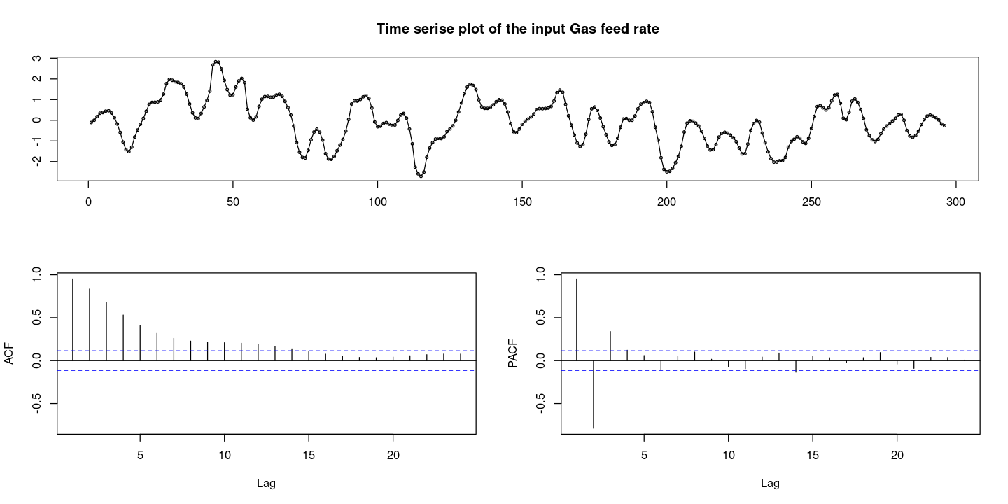
0을 기준으로 대칭인 것 처럼 보이고 등분산도 만족해 보인다. —> 정상시계열 같다.
결정적 추세는 없다.
ACF를 보면 확률적 추세가 있다면 천천히 감소하지만, 이건 지수적으로 감소하는 느낌이니까 확률적 추세가 있다고 하기엔 애매한 그림이다. 좀이따가 단위근 검정을 해보자.
PACF를 보면 3개만 살아있고 다 절단이다.
AR(3)모형이 적합해 보인다.
#모형 적합도 검정 : H0 : rho1=...=rho_k=0 : 포투맨트검정 : rate 가 백색잡음 과정인가?
Box.test(dt$rate, lag=1, type = "Ljung-Box")
Box.test(dt$rate, lag=6, type = "Ljung-Box") #rho1=rho2=...=rho6=0
Box.test(dt$rate, lag=12, type = "Ljung-Box") #rho1=...=rho12=0
    Box-Ljung test

data:  dt$rate
X-squared = 271.26, df = 1, p-value < 2.2e-16
    Box-Ljung test

data:  dt$rate
X-squared = 786.35, df = 6, p-value < 2.2e-16
    Box-Ljung test

data:  dt$rate
X-squared = 874.07, df = 12, p-value < 2.2e-16
H0를 기각하지 못하면 WN이다.
H0를 기각하면 WH가 아니니가 모형 적합을 해야한다.
H0를 다 기각함. 모두 다 0인건 아님. WN아니야!
- 단위근 검정
### random walk process 에서의 단위근 검정
z <- rnorm(100) #WN
cz <- cumsum(z) #random walkforecast::tsdisplay(z)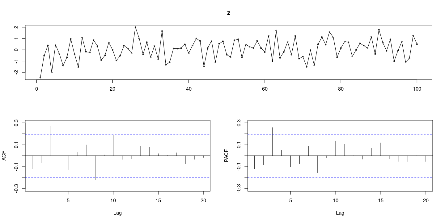
forecast::tsdisplay(cz)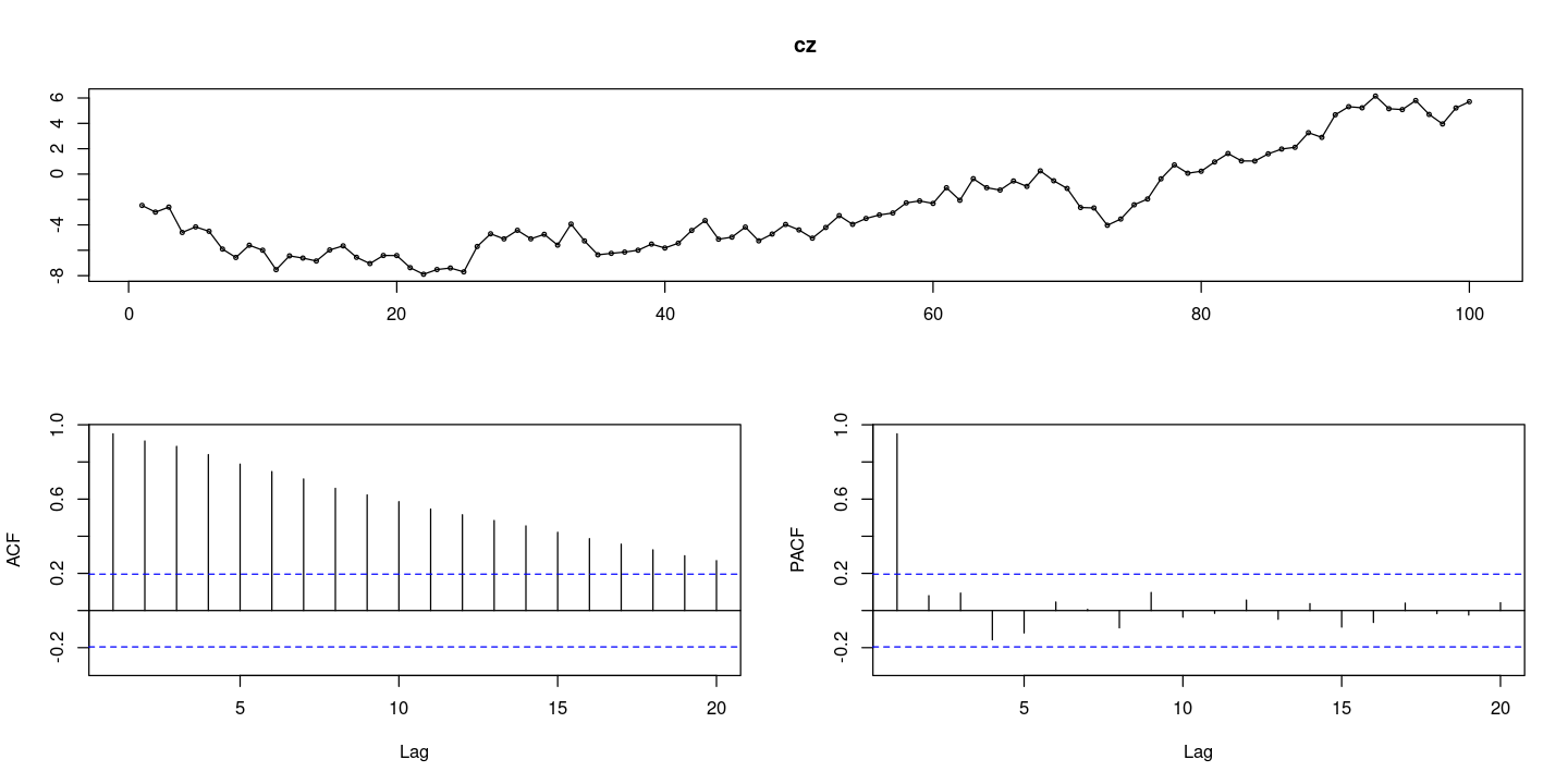
- ACF그래프가 천천히 감소한다.
fUnitRoots::adfTest(z, lags = 1, type = "nc")
#H0 : phi=1 단위근이 있다 , 차분이 필요하다. :(1-phi*B)Zt = et
#H1 : |rho|<1 단위근이 없다. 차분이 필요하지 않다.
Warning message in fUnitRoots::adfTest(z, lags = 1, type = "nc"):
“p-value smaller than printed p-value”
Title:
 Augmented Dickey-Fuller Test

Test Results:
  PARAMETER:
    Lag Order: 1
  STATISTIC:
    Dickey-Fuller: -8.2198
  P VALUE:
    0.01

Description:
 Tue Nov 28 22:16:00 2023 by user:
lags = 1 : 단위근이 1개 있는 거 보자
type: ‘nc’, ‘c’, ‘ct’ 3개가 있음
type = ‘nc’ : 가지고 있는 데이터가 평균이 0이면 이 옵션 사용
type = ‘c’ : 가지고 있는 데이터가 평균이 0이 아니면 이 옵션 사용 (상수항이 있는)
type = ‘ct’ : 결정적 추세가 있어 보이면 이 옵션 사용 (ㅅ상수항과 기울기가 있는)
WN이니까 차분이 필요하면 안되겠지? —> pvalue값이 작아. 기각 ㄱㄱ
fUnitRoots::adfTest(cz, lags = 0, type = "nc") #H0 : phi=1
fUnitRoots::adfTest(cz, lags = 1, type = "nc") #H0 : phi=1
fUnitRoots::adfTest(cz, lags = 2, type = "nc") #H0 : phi=1
#H0 : phi=1 단위근이 있다 , 차분이 필요하다. :(1-phi*B)Zt = et
#H1 : |rho|<1 단위근이 없다. 차분이 필요하지 않다.
Title:
 Augmented Dickey-Fuller Test

Test Results:
  PARAMETER:
    Lag Order: 0
  STATISTIC:
    Dickey-Fuller: -0.5717
  P VALUE:
    0.4309

Description:
 Tue Nov 28 22:19:33 2023 by user:
Title:
 Augmented Dickey-Fuller Test

Test Results:
  PARAMETER:
    Lag Order: 1
  STATISTIC:
    Dickey-Fuller: -0.4404
  P VALUE:
    0.4728

Description:
 Tue Nov 28 22:19:33 2023 by user:
Title:
 Augmented Dickey-Fuller Test

Test Results:
  PARAMETER:
    Lag Order: 2
  STATISTIC:
    Dickey-Fuller: -0.3474
  P VALUE:
    0.5024

Description:
Tue Nov 28 22:19:33 2023 by user: - pvalue가 애매하게 되었따. 0.05로 주면 기각할 수 있지만 0.01이면 기각 못함..
## 단위근 검정 H0 : 단위근이 있다.
## 상수항, 추세 (nc, c, ct)
fUnitRoots::adfTest(dt$rate, lags = 1, type = "nc")
Warning message in fUnitRoots::adfTest(dt$rate, lags = 1, type = "nc"):
“p-value smaller than printed p-value”
Title:
 Augmented Dickey-Fuller Test

Test Results:
  PARAMETER:
    Lag Order: 1
  STATISTIC:
    Dickey-Fuller: -7.6608
  P VALUE:
    0.01

Description:
Tue Nov 28 22:21:39 2023 by user: - 기각을 해버리자 —> 단위근 없다 —> 차분 필요 없다.
- 평균 포함
## 평균 포함
mean(dt$rate)
-0.0568344594594595
- 거의 0에 가깝다.
t.test(dt$rate) # H0 : mu=0
    One Sample t-test

data:  dt$rate
t = -0.91149, df = 295, p-value = 0.3628
alternative hypothesis: true mean is not equal to 0
95 percent confidence interval:
 -0.17954799  0.06587907
sample estimates:
  mean of x
-0.05683446 - pvalue가 0.3이 되서 H0를 기각 못한다. 즉 mu=0이다.
- arima
# ?arimainclude.mean = TRUE: default가 true이다.fixed= AR()모형으로 픽스할래 ! 이런식으로 할 때init= 초기값 설정
- 모형 적합 : AR(3)
\(X_t = a_1X_{t−1} + ⋯ + a_pX_{t−p} + e_t + b_1e_{t−1} + ⋯ + b_qe_{t−q}\) : e앞에 부호 조심!
## 모형 적합
fit1 <- arima(dt$rate, order=c(3,0,0)) #method = c("CSS-ML", "ML", "CSS")
#default method: to use CLSE to find starting values, then ML
fit1
# intercept = mu
Call:
arima(x = dt$rate, order = c(3, 0, 0))

Coefficients:
         ar1      ar2     ar3  intercept
      1.9691  -1.3651  0.3394    -0.0606
s.e.  0.0544   0.0985  0.0543     0.1898

sigma^2 estimated as 0.0353: log likelihood = 72.57, aic = -135.14summary(fit1)
Call:
arima(x = dt$rate, order = c(3, 0, 0))

Coefficients:
         ar1      ar2     ar3  intercept
      1.9691  -1.3651  0.3394    -0.0606
s.e.  0.0544   0.0985  0.0543     0.1898

sigma^2 estimated as 0.0353:  log likelihood = 72.57,  aic = -135.14

Training set error measures:
                       ME      RMSE       MAE MPE MAPE      MASE        ACF1
Training set 3.004966e-05 0.1878719 0.1307624 NaN  Inf 0.5140648 -0.03522643
- 통계적 유의성 확인하려고 할 때: coeftest
lmtest::coeftest(fit1)
z test of coefficients:

           Estimate Std. Error  z value  Pr(>|z|)
ar1        1.969066   0.054385  36.2061 < 2.2e-16 ***
ar2       -1.365143   0.098538 -13.8540 < 2.2e-16 ***
ar3        0.339404   0.054328   6.2473 4.177e-10 ***
intercept -0.060643   0.189800  -0.3195    0.7493
---
Signif. codes: 0 ‘***’ 0.001 ‘**’ 0.01 ‘*’ 0.05 ‘.’ 0.1 ‘ ’ 1- ph1, ph2, ph3는 다 유의하다. intercept(평균)은 별로 유이하지 않아.
fit2 <- arima(dt$rate, order=c(3,0,0), include.mean = F) # 위에서 평균은 유의하지 않았으므로 평균 빼고 다시 적합
summary(fit2)
Call:
arima(x = dt$rate, order = c(3, 0, 0), include.mean = F)

Coefficients:
         ar1      ar2     ar3
      1.9696  -1.3659  0.3399
s.e.  0.0544   0.0985  0.0543

sigma^2 estimated as 0.03531:  log likelihood = 72.52,  aic = -137.04

Training set error measures:
                       ME      RMSE       MAE MPE MAPE      MASE        ACF1
Training set -0.003418121 0.1879034 0.1305995 NaN Inf 0.5134245 -0.03583041- AIC가 감소했으므로 mean을 뺀게 더 유의한 모형
lmtest::coeftest(fit2)
z test of coefficients:

     Estimate Std. Error  z value  Pr(>|z|)
ar1  1.969560   0.054371  36.2243 < 2.2e-16 ***
ar2 -1.365925   0.098522 -13.8641 < 2.2e-16 ***
ar3  0.339906   0.054314   6.2582 3.894e-10 ***
---
Signif. codes: 0 ‘***’ 0.001 ‘**’ 0.01 ‘*’ 0.05 ‘.’ 0.1 ‘ ’ 1ls(fit1)- 'aic'
- 'arma'
- 'call'
- 'code'
- 'coef'
- 'loglik'
- 'mask'
- 'model'
- 'n.cond'
- 'nobs'
- 'residuals'
- 'series'
- 'sigma2'
- 'var.coef'
fit1$aic
fit2$aic
-135.137805258848
-137.035703041016
fit2$sigma2 # 오차의 분산에 대한 추정량
0.0353076789684466
- 잠정모형 : AR(3)
\(Z_t = 1.97Z_{t−1} − 1.37Z_{t−2} + 0.34Z_{t−3} + ε_t\)
\(\hatσ^2 = 0.0353\)
- 잔차분석
resid = resid(fit2)
forecast::tsdisplay(resid)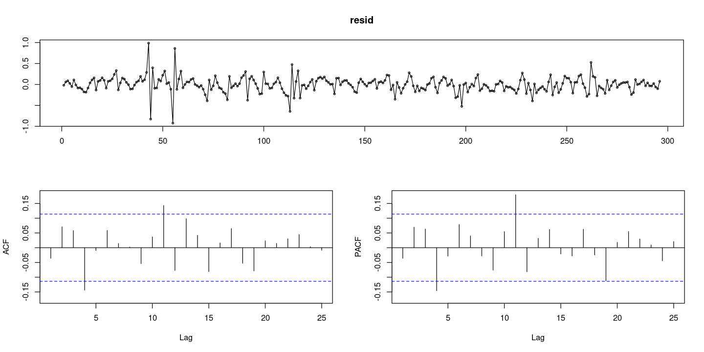
- 잔차의 정규성 검정
## 정규성검정
tseries::jarque.bera.test(resid) ##JB test H0: normal distribution
    Jarque Bera Test

data:  resid
X-squared = 496.68, df = 2, p-value < 2.2e-16par(mfrow=c(1,2))
hist(resid)
qqnorm(resid, pch=16)
qqline(resid)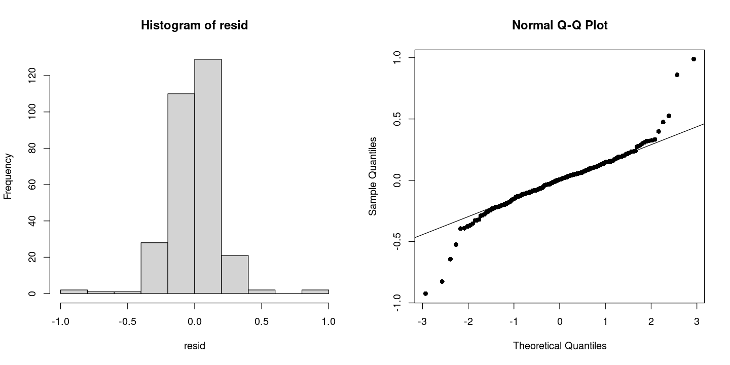
- 꼬리가 엄청 두껍다. 정규분포 ㄴㄴ같은데? 근데 책에서는 몇개 튀어나온 5개 점 때문에 그런거니까 그거 빼곤 정규분포 같아~ 라구 하기도 한다.
# 잔차의 포트맨토 검정 ## H0 : rho1=...=rho_k=0
portes::LjungBox(fit2, lags=c(6,12,18,24))| lags | statistic | df | p-value | |
|---|---|---|---|---|
| 6 | 10.21058 | 3 | 0.01685835 | |
| 12 | 19.76879 | 9 | 0.01939412 | |
| 18 | 27.70650 | 15 | 0.02348012 | |
| 24 | 30.86553 | 21 | 0.07592519 |
6번째깢/ 12번째까지/ 18번쨰까지/ 24번쨰까지 싹 다 0인지 보여줘!
이상점 때문에 pvalue값이 애매하게 나옴
## 잔차 검정
astsa::sarima(dt$rate, p=3, d=0, q=1)initial value 0.073551
iter 2 value -0.073322
iter 3 value -0.178255
iter 4 value -0.376823
iter 5 value -0.612419
iter 6 value -0.918313
iter 7 value -1.297243
iter 8 value -1.540430
iter 9 value -1.547244
iter 10 value -1.619914
iter 11 value -1.629287
iter 12 value -1.632509
iter 13 value -1.632906
iter 14 value -1.633608
iter 15 value -1.635745
iter 16 value -1.637069
iter 17 value -1.637183
iter 18 value -1.637941
iter 19 value -1.638469
iter 20 value -1.639157
iter 21 value -1.645795
iter 22 value -1.654637
iter 23 value -1.659278
iter 24 value -1.667888
iter 25 value -1.672991
iter 26 value -1.674756
iter 27 value -1.675067
iter 28 value -1.675120
iter 29 value -1.675335
iter 30 value -1.675343
iter 31 value -1.675347
iter 32 value -1.675363
iter 33 value -1.675371
iter 34 value -1.675374
iter 35 value -1.675374
iter 35 value -1.675374
iter 35 value -1.675374
final value -1.675374
converged
initial value -1.671802
iter 2 value -1.671805
iter 3 value -1.671828
iter 4 value -1.671829
iter 5 value -1.671833
iter 6 value -1.671834
iter 7 value -1.671837
iter 8 value -1.671837
iter 9 value -1.671838
iter 10 value -1.671838
iter 11 value -1.671838
iter 12 value -1.671839
iter 13 value -1.671839
iter 14 value -1.671839
iter 14 value -1.671839
iter 14 value -1.671839
final value -1.671839
converged$fit
Call:
arima(x = xdata, order = c(p, d, q), seasonal = list(order = c(P, D, Q), period = S),
xreg = xmean, include.mean = FALSE, transform.pars = trans, fixed = fixed,
optim.control = list(trace = trc, REPORT = 1, reltol = tol))
Coefficients:
ar1 ar2 ar3 ma1 xmean
2.2497 -1.8431 0.5607 -0.3203 -0.0593
s.e. 0.1158 0.1954 0.0909 0.1344 0.2202
sigma^2 estimated as 0.03475: log likelihood = 74.86, aic = -137.72
$degrees_of_freedom
[1] 291
$ttable
Estimate SE t.value p.value
ar1 2.2497 0.1158 19.4217 0.0000
ar2 -1.8431 0.1954 -9.4338 0.0000
ar3 0.5607 0.0909 6.1657 0.0000
ma1 -0.3203 0.1344 -2.3830 0.0178
xmean -0.0593 0.2202 -0.2694 0.7878
$AIC
[1] -0.4652596
$AICc
[1] -0.4645607
$BIC
[1] -0.390455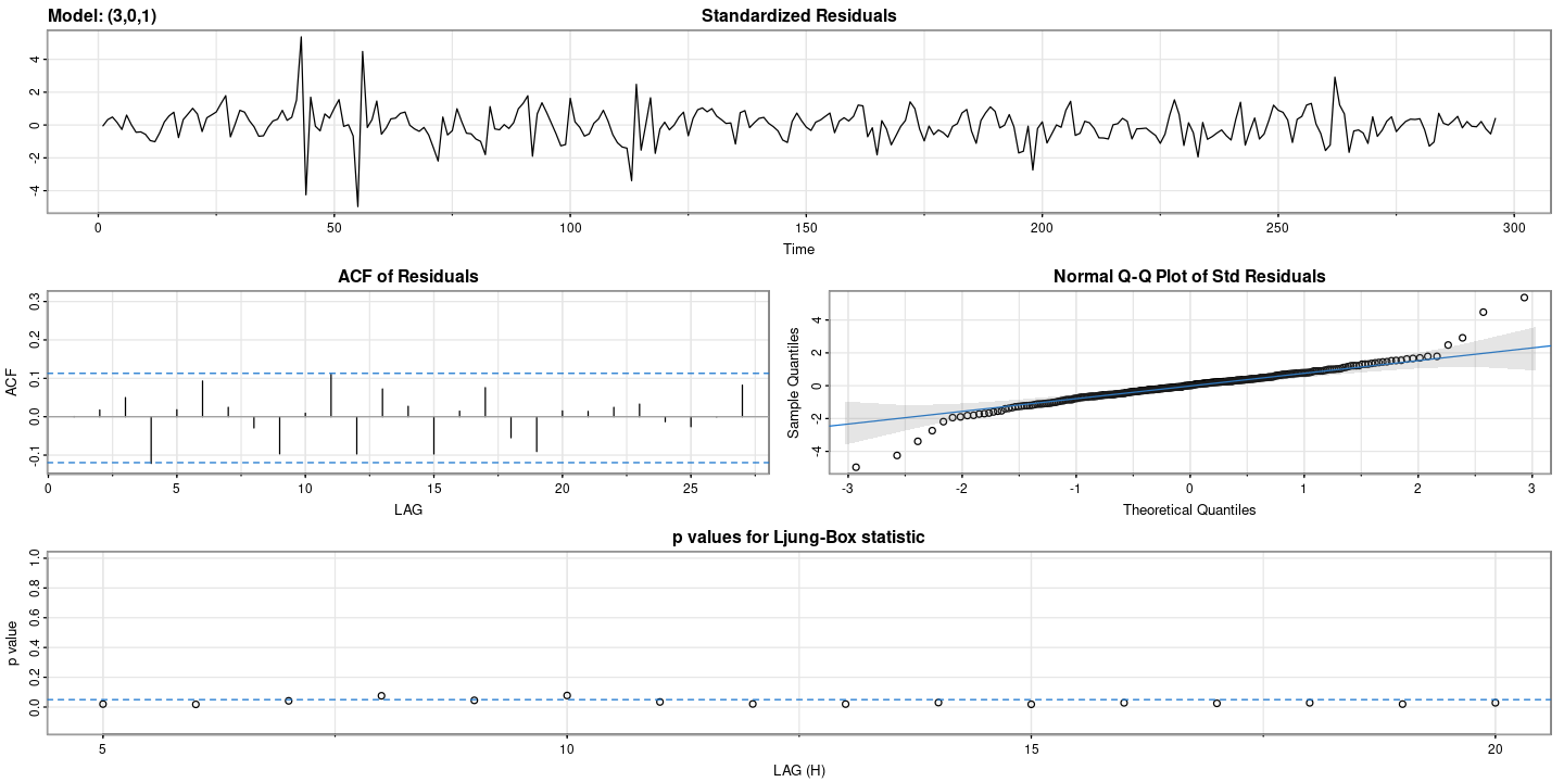
astsa::sarima(dt$rate, p=3, d=0, q=1, details=F)$fit
Call:
arima(x = xdata, order = c(p, d, q), seasonal = list(order = c(P, D, Q), period = S),
xreg = xmean, include.mean = FALSE, transform.pars = trans, fixed = fixed,
optim.control = list(trace = trc, REPORT = 1, reltol = tol))
Coefficients:
ar1 ar2 ar3 ma1 xmean
2.2497 -1.8431 0.5607 -0.3203 -0.0593
s.e. 0.1158 0.1954 0.0909 0.1344 0.2202
sigma^2 estimated as 0.03475: log likelihood = 74.86, aic = -137.72
$degrees_of_freedom
[1] 291
$ttable
Estimate SE t.value p.value
ar1 2.2497 0.1158 19.4217 0.0000
ar2 -1.8431 0.1954 -9.4338 0.0000
ar3 0.5607 0.0909 6.1657 0.0000
ma1 -0.3203 0.1344 -2.3830 0.0178
xmean -0.0593 0.2202 -0.2694 0.7878
$AIC
[1] -0.4652596
$AICc
[1] -0.4645607
$BIC
[1] -0.390455# 12시차 앞에 것을 예측해줘!!!
astsa::sarima.for(dt$rate, n.ahead=12, p=3, d=0, q=0)- $pred
- A Time Series:
- -0.265106139192775
- -0.229552377440341
- -0.182456715763015
- -0.139312468943022
- -0.106583819040958
- -0.0850525454735895
- -0.0726919904363936
- -0.0666382629913424
- -0.0642841907844162
- -0.063717844077476
- -0.0637616533051378
- -0.0638220781876669
- $se
- A Time Series:
- 0.187871938724622
- 0.414904448800112
- 0.628395849359732
- 0.795661017554752
- 0.910326093209164
- 0.98070415660671
- 1.01994737390418
- 1.04011443482053
- 1.04985151276616
- 1.05439175132729
- 1.05651197077771
- 1.05754419307717
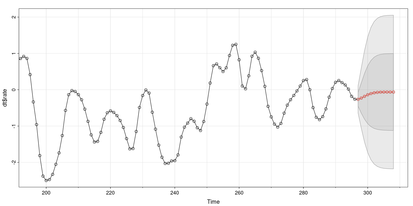
- 신뢰구간 까지 구해준다. 신기하군..
- 과대적합을 해 볼 수도 있음 : AR(4), AR(3,1)
fit2 <- arima(dt$rate, order=c(3,0,0)) #AR(3)
fit3 <- arima(dt$rate, order=c(4,0,0)) #AR(4)
fit4 <- arima(dt$rate, order=c(3,0,1)) #ARMA(3,1)
fit5 <- arima(dt$rate, order=c(4,0,1)) #ARMA(4,1)lmtest::coeftest(fit2)
lmtest::coeftest(fit3)
lmtest::coeftest(fit4)
lmtest::coeftest(fit5)
z test of coefficients:
Estimate Std. Error z value Pr(>|z|)
ar1 1.969066 0.054385 36.2061 < 2.2e-16 ***
ar2 -1.365143 0.098538 -13.8540 < 2.2e-16 ***
ar3 0.339404 0.054328 6.2473 4.177e-10 ***
intercept -0.060643 0.189800 -0.3195 0.7493
---
Signif. codes: 0 ‘***’ 0.001 ‘**’ 0.01 ‘*’ 0.05 ‘.’ 0.1 ‘ ’ 1
z test of coefficients:
Estimate Std. Error z value Pr(>|z|)
ar1 1.927075 0.057476 33.5284 < 2e-16 ***
ar2 -1.197232 0.125870 -9.5116 < 2e-16 ***
ar3 0.098632 0.125831 0.7838 0.43313
ar4 0.121539 0.057377 2.1183 0.03415 *
intercept -0.059332 0.212340 -0.2794 0.77992
---
Signif. codes: 0 ‘***’ 0.001 ‘**’ 0.01 ‘*’ 0.05 ‘.’ 0.1 ‘ ’ 1
z test of coefficients:
Estimate Std. Error z value Pr(>|z|)
ar1 2.249705 0.115834 19.4217 < 2.2e-16 ***
ar2 -1.843111 0.195373 -9.4338 < 2.2e-16 ***
ar3 0.560735 0.090945 6.1657 7.019e-10 ***
ma1 -0.320319 0.134416 -2.3830 0.01717 *
intercept -0.059321 0.220225 -0.2694 0.78765
---
Signif. codes: 0 ‘***’ 0.001 ‘**’ 0.01 ‘*’ 0.05 ‘.’ 0.1 ‘ ’ 1
z test of coefficients:
Estimate Std. Error z value Pr(>|z|)
ar1 2.095578 0.310005 6.7598 1.382e-11 ***
ar2 -1.527029 0.618747 -2.4679 0.01359 *
ar3 0.324392 0.445860 0.7276 0.46688
ar4 0.066838 0.123362 0.5418 0.58795
ma1 -0.172334 0.307391 -0.5606 0.57505
intercept -0.057957 0.217926 -0.2659 0.79028
---
Signif. codes: 0 ‘***’ 0.001 ‘**’ 0.01 ‘*’ 0.05 ‘.’ 0.1 ‘ ’ 1AR(4)와 AR(3)을 비교해 보면, AR(4)에서는 ar4가 유의하긴 하지만.. *한개라서 선택안하는게 나을 듯 하다.
ARMA(3,0,1)도 그닥
ARMA(4,0,1) 공통인수가 생겨서 더 이상해졌다.
paste0("AIC for AR(3) = ", fit2$aic)
paste0("AIC for AR(4) = ", fit3$aic)
paste0("AIC for ARMA(3,1) = ", fit4$aic)
paste0("AIC for ARMA(4,1) = ", fit5$aic)
'AIC for AR(3) = -135.137805258848'
'AIC for AR(4) = -137.587994248135'
'AIC for ARMA(3,1) = -137.71684916351'
'AIC for ARMA(4,1) = -135.941477951932'
- auto.aroma
- 자동으로 좋은거 찾아줘
forecast::auto.arima(dt$rate, ic='bic', test="adf", trace = T)
Fitting models using approximations to speed things up...
ARIMA(2,0,2) with non-zero mean : -108.9179
ARIMA(0,0,0) with non-zero mean : 891.9727
ARIMA(1,0,0) with non-zero mean : 194.5692
ARIMA(0,0,1) with non-zero mean : 520.7498
ARIMA(0,0,0) with zero mean : 887.1148
ARIMA(1,0,2) with non-zero mean : -68.83754
ARIMA(2,0,1) with non-zero mean : -109.6656
ARIMA(1,0,1) with non-zero mean : -11.98193
ARIMA(2,0,0) with non-zero mean : -88.26513
ARIMA(3,0,1) with non-zero mean : -117.6677
ARIMA(3,0,0) with non-zero mean : -118.7078
ARIMA(4,0,0) with non-zero mean : -116.5382
ARIMA(4,0,1) with non-zero mean : -111.1943
ARIMA(3,0,0) with zero mean : -124.2755
ARIMA(2,0,0) with zero mean : -93.73805
ARIMA(4,0,0) with zero mean : -122.1245
ARIMA(3,0,1) with zero mean : -123.2595
ARIMA(2,0,1) with zero mean : -115.215
ARIMA(4,0,1) with zero mean : -116.7881
Now re-fitting the best model(s) without approximations...
ARIMA(3,0,0) with zero mean : -122.2743
Best model: ARIMA(3,0,0) with zero mean
Series: dt$rate
ARIMA(3,0,0) with zero mean
Coefficients:
ar1 ar2 ar3
1.9696 -1.3659 0.3399
s.e. 0.0544 0.0985 0.0543
sigma^2 = 0.03567: log likelihood = 72.52
AIC=-137.04 AICc=-136.9 BIC=-122.27fit2$sigma2
0.0352958653601482
EX 8.7 모의 실험 데이터
z <- scan("eg8_7.txt")
forecast::tsdisplay(z)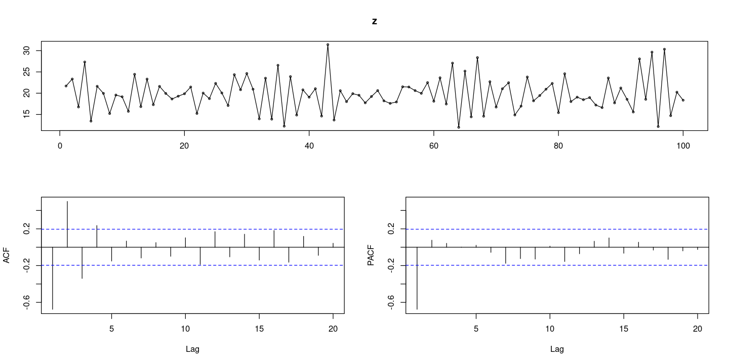
평균이 20정도 이고 추세나 계절성분이 보이지 않는 정상 시계열
acf는 사인 함수 형태를 그리며 지수적으로 감소하는 형태
pacf는 처음만 ㅏㅅㄹ아남고 나머지는 다 0인 AR(1)모형
#모형 적합도 검정 : H0 : rho1=...=rho_k=0 WN
Box.test(z, lag=1, type = "Ljung-Box")
Box.test(z, lag=6, type = "Ljung-Box")
Box.test(z, lag=12, type = "Ljung-Box")
Box-Ljung test
data: z
X-squared = 47.058, df = 1, p-value = 6.892e-12
Box-Ljung test
data: z
X-squared = 93.925, df = 6, p-value < 2.2e-16
Box-Ljung test
data: z
X-squared = 105.37, df = 12, p-value < 2.2e-16모든 시차에서 다 기각을 한다.
WN가 아니다.
## 단위근 검정 H0 : 단위근이 있다.
fUnitRoots::adfTest(z, lags = 0, type = "c")
fUnitRoots::adfTest(z, lags = 1, type = "c")
fUnitRoots::adfTest(z, lags = 2, type = "c")Warning message in fUnitRoots::adfTest(z, lags = 0, type = "c"):
“p-value smaller than printed p-value”
Warning message in fUnitRoots::adfTest(z, lags = 1, type = "c"):
“p-value smaller than printed p-value”
Warning message in fUnitRoots::adfTest(z, lags = 2, type = "c"):
“p-value smaller than printed p-value”
Title:
Augmented Dickey-Fuller Test
Test Results:
PARAMETER:
Lag Order: 0
STATISTIC:
Dickey-Fuller: -22.4468
P VALUE:
0.01
Description:
Tue Nov 28 22:50:24 2023 by user:
Title:
Augmented Dickey-Fuller Test
Test Results:
PARAMETER:
Lag Order: 1
STATISTIC:
Dickey-Fuller: -8.4607
P VALUE:
0.01
Description:
Tue Nov 28 22:50:24 2023 by user:
Title:
Augmented Dickey-Fuller Test
Test Results:
PARAMETER:
Lag Order: 2
STATISTIC:
Dickey-Fuller: -5.98
P VALUE:
0.01
Description:
Tue Nov 28 22:50:24 2023 by user: - 다 기각! 단위근이 없다. 차분을 할 필요가 없다.!!
## 모형적합 AR(1)
fit <- arima(z,order=c(1,0,0))
summary(fit)
Call:
arima(x = z, order = c(1, 0, 0))
Coefficients:
ar1 intercept
-0.6715 19.8312
s.e. 0.0728 0.1776
sigma^2 estimated as 8.744: log likelihood = -250.61, aic = 507.22
Training set error measures:
ME RMSE MAE MPE MAPE MASE
Training set 0.007670341 2.957007 2.337302 -2.080783 11.9899 0.4096807
ACF1
Training set 0.04344908ts.plot(z, fitted(fit), col=1:2, lty=1:2, lwd=2)
abline(h=mean(z), col="grey", lty=2)
legend("topleft", c("z", "fitted z"), col=1:2, lty=1:2)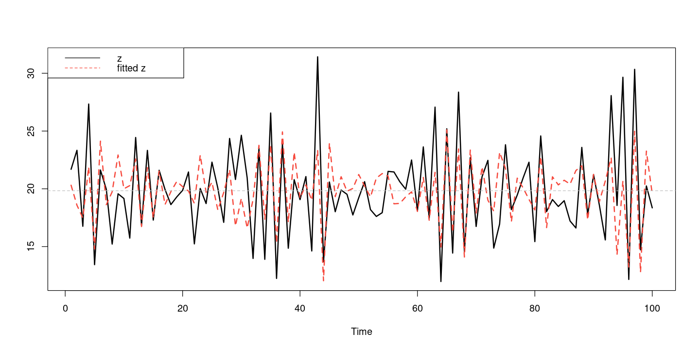
sum((z - fitted(fit))^2) #SSE
sum((z - fitted(fit))^2) / 100 #MSE
sqrt(sum((z - fitted(fit))^2) / 100) #RMSE
sum(abs(z-fitted(fit))/100) #MAE
sum(abs(z-fitted(fit))/z)*100/100 #MAPE
874.389110536135
8.74389110536135
2.95700711959937
2.337302165617
11.9898979348871
lmtest::coeftest(fit)
z test of coefficients:
Estimate Std. Error z value Pr(>|z|)
ar1 -0.671544 0.072838 -9.2197 < 2.2e-16 ***
intercept 19.831150 0.177618 111.6504 < 2.2e-16 ***
---
Signif. codes: 0 ‘***’ 0.001 ‘**’ 0.01 ‘*’ 0.05 ‘.’ 0.1 ‘ ’ 1fit$sigma2
8.74389110536135
(1-0.67)*19.83 # delta
6.5439
- AR(1)
\(Z_t − 19.83 = 0.67(Z_{t−1} − 19.83) + ε_t\)
\(Z_t = 6.54 + 0.67Z_{t−1} + ε_t\)
\(\hatσ^2 = 8.744\)
- 잔차분석
resid = resid(fit)
forecast::tsdisplay(resid)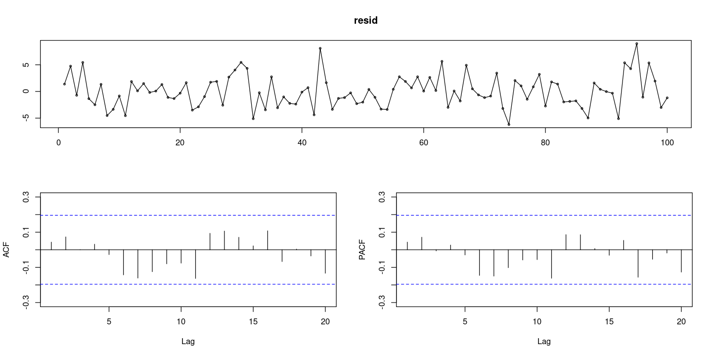
# 잔차의 포트맨토 검정 ## H0 : rho1=...=rho_k=0
portes::LjungBox(fit, lags=c(6,12,18,24))| lags | statistic | df | p-value | |
|---|---|---|---|---|
| 6 | 3.147291 | 5 | 0.6772898 | |
| 12 | 13.135047 | 11 | 0.2845906 | |
| 18 | 17.072699 | 17 | 0.4494514 | |
| 24 | 24.393987 | 23 | 0.3822679 |
- H0기각 못함. 다 0이다! WN이다.
## 정규성검정
tseries::jarque.bera.test(resid) ##JB test H0: norma
Jarque Bera Test
data: resid
X-squared = 4.2649, df = 2, p-value = 0.1185par(mfrow=c(1,2))
hist(resid)
qqnorm(resid, pch=16)
qqline(resid)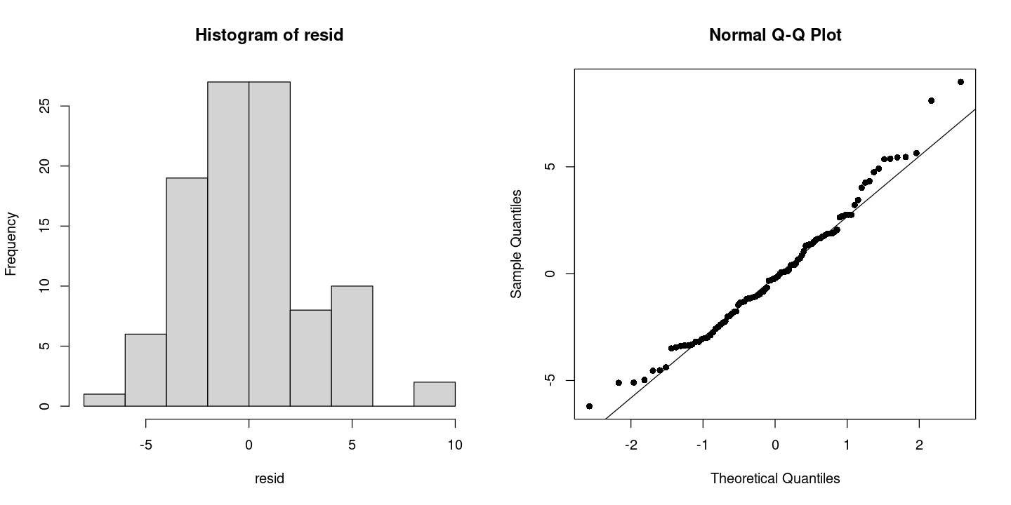
- 정규분포이다.
## 잔차 검정
astsa::sarima(z, p=1, d=0, q=0)initial value 1.394650
iter 2 value 1.088119
iter 3 value 1.088089
iter 4 value 1.088089
iter 5 value 1.088089
iter 5 value 1.088089
iter 5 value 1.088089
final value 1.088089
converged
initial value 1.087203
iter 2 value 1.087196
iter 3 value 1.087176
iter 4 value 1.087176
iter 4 value 1.087176
iter 4 value 1.087176
final value 1.087176
converged$fit
Call:
arima(x = xdata, order = c(p, d, q), seasonal = list(order = c(P, D, Q), period = S),
xreg = xmean, include.mean = FALSE, transform.pars = trans, fixed = fixed,
optim.control = list(trace = trc, REPORT = 1, reltol = tol))
Coefficients:
ar1 xmean
-0.6715 19.8312
s.e. 0.0728 0.1776
sigma^2 estimated as 8.744: log likelihood = -250.61, aic = 507.22
$degrees_of_freedom
[1] 98
$ttable
Estimate SE t.value p.value
ar1 -0.6715 0.0728 -9.2197 0
xmean 19.8312 0.1776 111.6504 0
$AIC
[1] 5.072228
$AICc
[1] 5.073466
$BIC
[1] 5.150384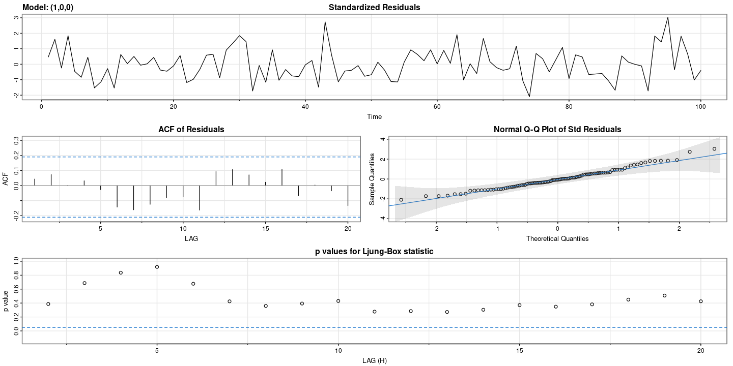
astsa::sarima.for(z, n.ahead=12, p=1, d=0, q=0)- $pred
- A Time Series:
- 20.8222483489762
- 19.1655839559512
- 20.2781070098918
- 19.5309988141942
- 20.032714849742
- 19.6957904500696
- 19.9220500133516
- 19.7701067583474
- 19.8721433414928
- 19.8036212850204
- 19.849636861772
- 19.8187353767205
- $se
- A Time Series:
- 2.95700711959937
- 3.5619005566917
- 3.80334404182832
- 3.90734998536685
- 3.95335857242263
- 3.97393285636323
- 3.98317649989949
- 3.98733810739122
- 3.98921345277822
- 3.99005889146209
- 3.99044010149264
- 3.9906120043846
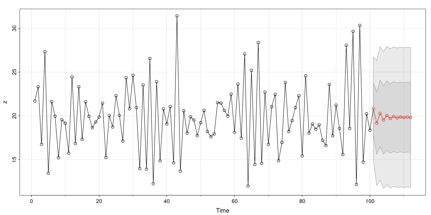
- 과대적합 AR(2), ARMA(1,1)
fit1 <- arima(z,order=c(1,0,0)) #AR(1)
fit2 <- arima(z,order=c(2,0,0)) #AR(2)
fit3 <- arima(z,order=c(1,0,1)) #ARMA(1,1)lmtest::coeftest(fit1)
z test of coefficients:
Estimate Std. Error z value Pr(>|z|)
ar1 -0.671544 0.072838 -9.2197 < 2.2e-16 ***
intercept 19.831150 0.177618 111.6504 < 2.2e-16 ***
---
Signif. codes: 0 ‘***’ 0.001 ‘**’ 0.01 ‘*’ 0.05 ‘.’ 0.1 ‘ ’ 1lmtest::coeftest(fit2)
z test of coefficients:
Estimate Std. Error z value Pr(>|z|)
ar1 -0.623116 0.100156 -6.2215 4.925e-10 ***
ar2 0.070388 0.100264 0.7020 0.4827
intercept 19.833114 0.190583 104.0657 < 2.2e-16 ***
---
Signif. codes: 0 ‘***’ 0.001 ‘**’ 0.01 ‘*’ 0.05 ‘.’ 0.1 ‘ ’ 1- ar2가 유의하지 앟네? 없어도 된다.
lmtest::coeftest(fit3)
z test of coefficients:
Estimate Std. Error z value Pr(>|z|)
ar1 -0.721425 0.097566 -7.3942 1.423e-13 ***
ma1 0.092687 0.139500 0.6644 0.5064
intercept 19.832916 0.187938 105.5291 < 2.2e-16 ***
---
Signif. codes: 0 ‘***’ 0.001 ‘**’ 0.01 ‘*’ 0.05 ‘.’ 0.1 ‘ ’ 1- 얘도 추가한게 의미가 없다리
paste0("AIC for AR(1) = ", fit1$aic)
paste0("AIC for AR(2) = ", fit2$aic)
paste0("AIC for ARMA(1,1) = ", fit3$aic)
'AIC for AR(1) = 507.222841029181'
'AIC for AR(2) = 508.731382853541'
'AIC for ARMA(1,1) = 508.786741594701'
fit1$sigma2
fit2$sigma2
fit3$sigma2
8.74389110536135
8.70042443220835
8.70536117214485
- 자유도를 고려하지 않기 때문에 크게 차이는 없ㅈ만.. 선택할 필요는 없다.
forecast::auto.arima(z, trace = T)
ARIMA(2,0,2) with non-zero mean : 513.4708
ARIMA(0,0,0) with non-zero mean : 566.0505
ARIMA(1,0,0) with non-zero mean : 507.4728
ARIMA(0,0,1) with non-zero mean : 529.1392
ARIMA(0,0,0) with zero mean : 887.3166
ARIMA(2,0,0) with non-zero mean : 509.1524
ARIMA(1,0,1) with non-zero mean : 509.2078
ARIMA(2,0,1) with non-zero mean : 511.2473
ARIMA(1,0,0) with zero mean : 686.5421
Best model: ARIMA(1,0,0) with non-zero mean
Series: z
ARIMA(1,0,0) with non-zero mean
Coefficients:
ar1 mean
-0.6715 19.8312
s.e. 0.0728 0.1776
sigma^2 = 8.922: log likelihood = -250.61
AIC=507.22 AICc=507.47 BIC=515.04EX 8.8 : 주가지수
z <- scan("elecstock.txt")
forecast::tsdisplay(z)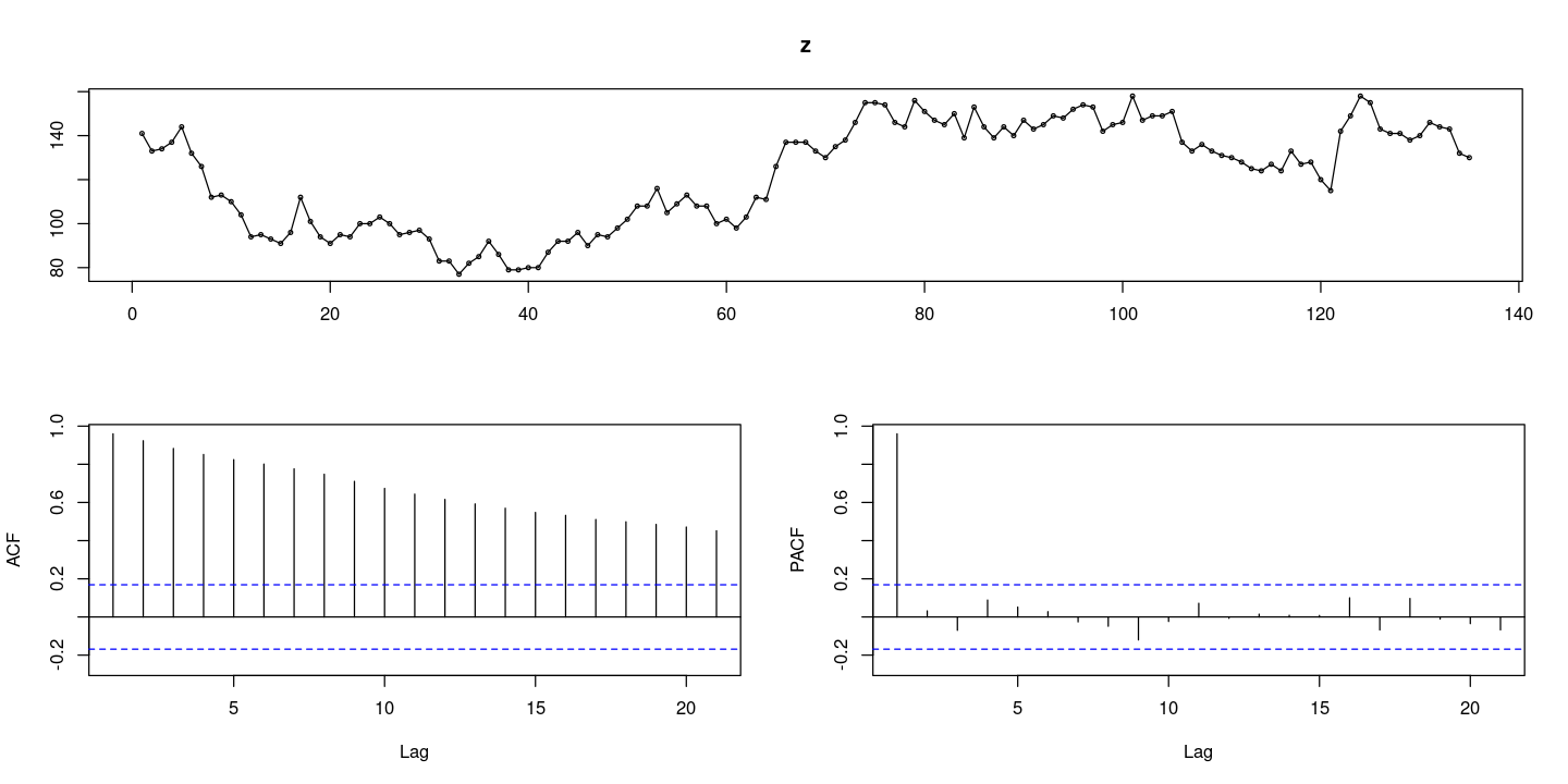
추세는 있으나 결정적 추세가 아닌 확률적 추세가 있어 보인다..
acf는 서서히 감소하고 pacf는 첫번째만 있는 거 보니 차분이 필요해 보이낟.
## 단위근 검정 H0 : 단위근이 있다.(phi=1) H1 : |phi|<1
fUnitRoots::adfTest(z, lags = 0, type = "c")
fUnitRoots::adfTest(z, lags = 1, type = "c")
fUnitRoots::adfTest(z, lags = 2, type = "c")
Title:
Augmented Dickey-Fuller Test
Test Results:
PARAMETER:
Lag Order: 0
STATISTIC:
Dickey-Fuller: -1.6769
P VALUE:
0.434
Description:
Tue Nov 28 22:59:53 2023 by user:
Title:
Augmented Dickey-Fuller Test
Test Results:
PARAMETER:
Lag Order: 1
STATISTIC:
Dickey-Fuller: -1.5572
P VALUE:
0.4784
Description:
Tue Nov 28 22:59:53 2023 by user:
Title:
Augmented Dickey-Fuller Test
Test Results:
PARAMETER:
Lag Order: 2
STATISTIC:
Dickey-Fuller: -1.629
P VALUE:
0.4517
Description:
Tue Nov 28 22:59:53 2023 by user: 기각을 못한다!! 차분이 필요해.
평균이 0이 아니니까 type=c 쓰는거 주의하자.
- 위의 함수 외에도 단위근 검정 함수는 아래 더 있음.
tseries::adf.test(z)
Augmented Dickey-Fuller Test
data: z
Dickey-Fuller = -2.6174, Lag order = 5, p-value = 0.3197
alternative hypothesis: stationarytseries::pp.test(z)
Phillips-Perron Unit Root Test
data: z
Dickey-Fuller Z(alpha) = -10.981, Truncation lag parameter = 4, p-value
= 0.4825
alternative hypothesis: stationary## 차분
diff_z = diff(z)
forecast::tsdisplay(diff_z)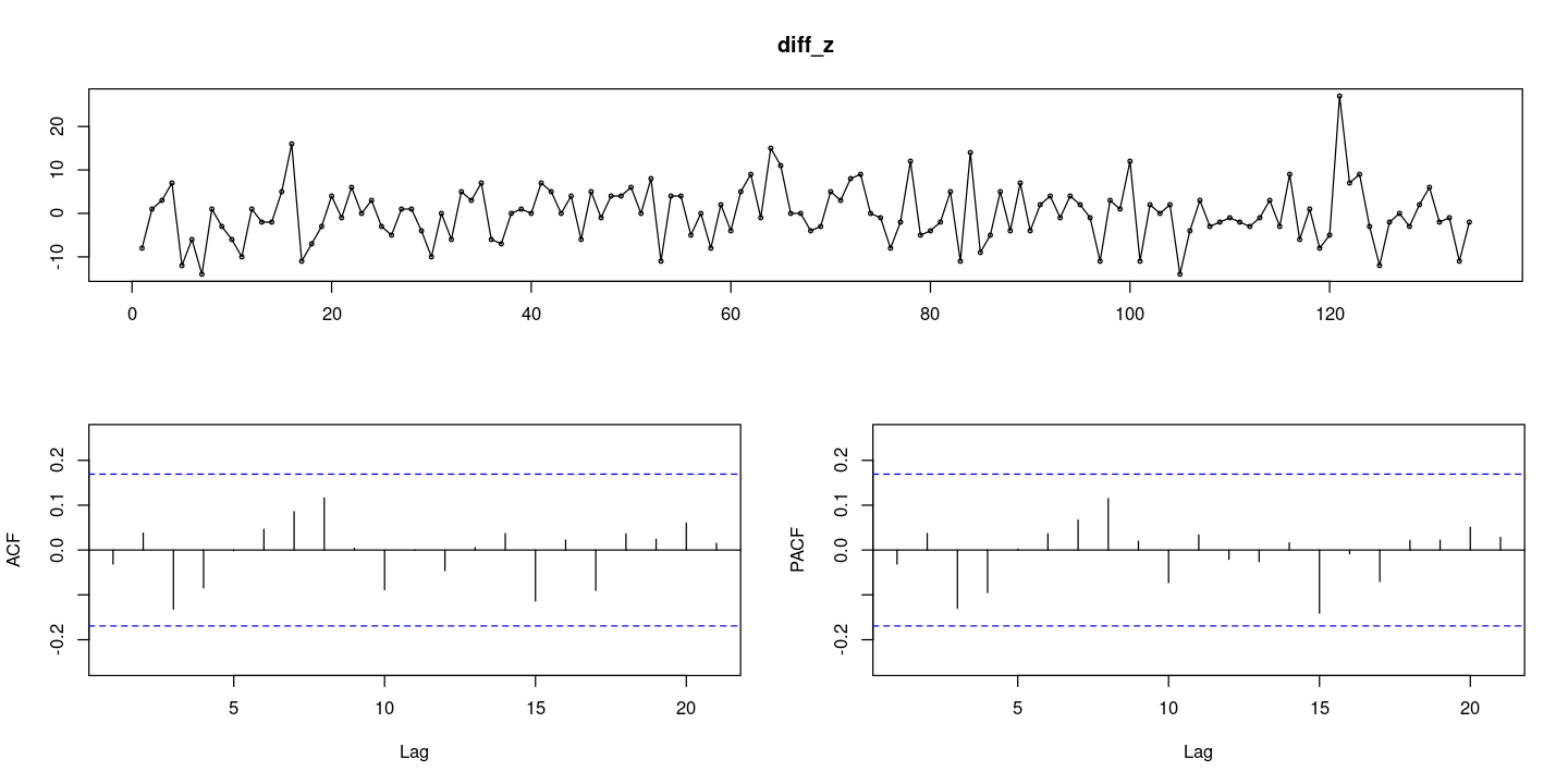
차분을 했더니 0을 중심으로 움직이고 있다..
acf/pacf 모든 차수에서 다 0이니까 WN이다! 엇, 그럼 랜덤워크네?
## 포투맨트검정 H0 : rho1=...=rho_k=0
Box.test(diff_z, lag=6, type = "Ljung-Box")
Box.test(diff_z, lag=12, type = "Ljung-Box")
Box-Ljung test
data: diff_z
X-squared = 4.0392, df = 6, p-value = 0.6714
Box-Ljung test
data: diff_z
X-squared = 8.5057, df = 12, p-value = 0.7445- 기각을 못한다. WN이다.
#평균
t.test(diff_z)
One Sample t-test
data: diff_z
t = -0.14564, df = 133, p-value = 0.8844
alternative hypothesis: true mean is not equal to 0
95 percent confidence interval:
-1.196970 1.032791
sample estimates:
mean of x
-0.08208955 평균이 0이라고 할 수 있다.
\(ΔZ_t ∼ WN(0, σ^2) ⇒ ΔZ_t ∼ ARIMA(0, 0, 0)\)
따라서, \(Z_t ∼ ARIMA(0, 1, 0)\)
## 모형적합 ARIMA(0,1,0)
fit <- arima(z,order=c(0,1,0))
summary(fit)
Call:
arima(x = z, order = c(0, 1, 0))
sigma^2 estimated as 42.26: log likelihood = -440.98, aic = 883.95
Training set error measures:
ME RMSE MAE MPE MAPE MASE
Training set -0.08043704 6.47675 4.897341 -0.2029409 4.084668 0.9928043
ACF1
Training set -0.03158845fit$sigma2
42.2611940298549
\(\hat σ^2 = 42.261\)
### 잔차검정
resid <- resid(fit)
forecast::tsdisplay(resid)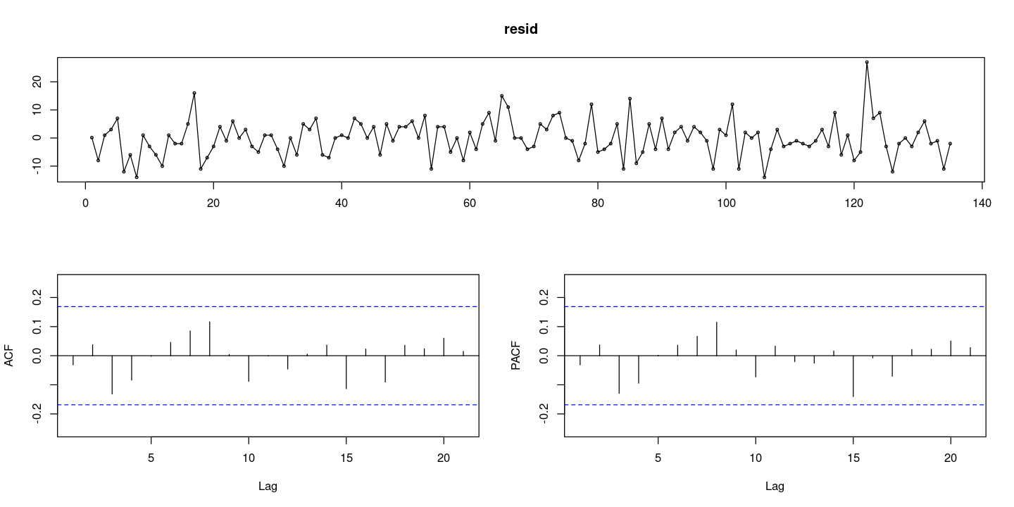
## 정규성검정
tseries::jarque.bera.test(resid) ##JB test H0: normal
Jarque Bera Test
data: resid
X-squared = 19.063, df = 2, p-value = 7.254e-05- 유의확률이 작게 나와서 정규분포라 하기는 어렵다.. (이상점 떄문에 꼬리)
par(mfrow=c(1,2))
hist(resid)
qqnorm(resid, pch=16)
qqline(resid)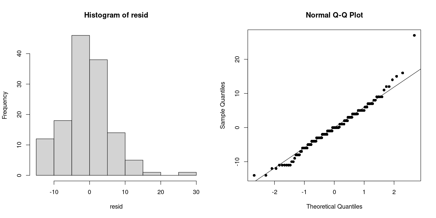
# 잔차의 포트맨토 검정 ## H0 : rho1=...=rho_k=0
portes::LjungBox(fit, lags=c(6,12,18,24))| lags | statistic | df | p-value | |
|---|---|---|---|---|
| 6 | 4.057476 | 6 | 0.6688985 | |
| 12 | 8.548020 | 12 | 0.7409734 | |
| 18 | 12.308859 | 18 | 0.8308883 | |
| 24 | 17.491184 | 24 | 0.8269712 |
- 다 유의하지 않다. 따라서 WN이다.
## 잔차 검정
astsa::sarima(z, p=0, d=1, q=0)initial value 1.871855
iter 1 value 1.871855
final value 1.871855
converged
initial value 1.871855
iter 1 value 1.871855
final value 1.871855
converged$fit
Call:
arima(x = xdata, order = c(p, d, q), seasonal = list(order = c(P, D, Q), period = S),
xreg = constant, transform.pars = trans, fixed = fixed, optim.control = list(trace = trc,
REPORT = 1, reltol = tol))
Coefficients:
constant
-0.0821
s.e. 0.5615
sigma^2 estimated as 42.25: log likelihood = -440.97, aic = 885.93
$degrees_of_freedom
[1] 133
$ttable
Estimate SE t.value p.value
constant -0.0821 0.5615 -0.1462 0.884
$AIC
[1] 6.611438
$AICc
[1] 6.611664
$BIC
[1] 6.654689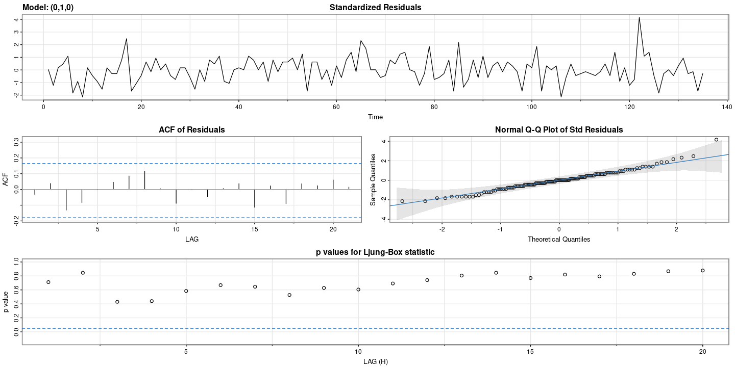
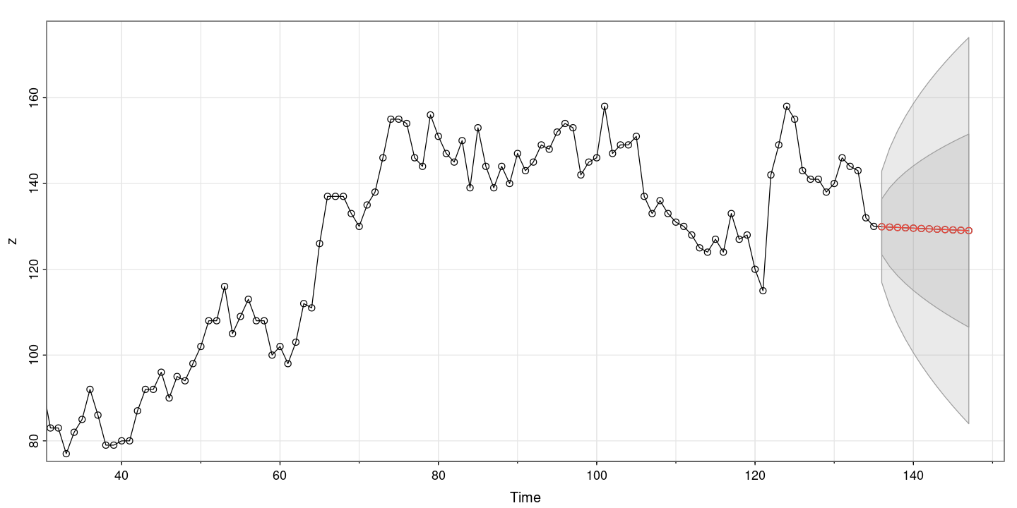
astsa::sarima.for(z, n.ahead=12, p=0, d=1, q=0)- $pred
- A Time Series:
- 129.917910447761
- 129.835820895522
- 129.753731343284
- 129.671641791045
- 129.589552238806
- 129.507462686567
- 129.425373134328
- 129.343283582089
- 129.261194029851
- 129.179104477612
- 129.097014925373
- 129.014925373134
- $se
- A Time Series:
- 6.50034270906296
- 9.1928728192299
- 11.258923838707
- 13.0006854181259
- 14.5352081745099
- 15.9225227904251
- 17.1982902448725
- 18.3857456384598
- 19.5010281271889
- 20.5558885323082
- 21.5591977746842
- 22.5178476774139
EX 8.9 : 여성근로자수
z <- scan("female.txt")
forecast::tsdisplay(z, main = "여성근로자 수의 시계열 그림과 SACF/SPACF")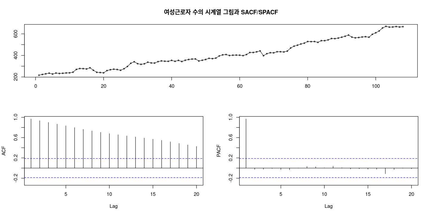
결정적 추세가 있어 보인다!
ACF: 천천히 감소.. —> 차분이 필요해!
PACF:처음만 살아있다.
## 단위근 검정 H0 : 단위근이 있다.
fUnitRoots::adfTest(z, lags = 0, type = "ct")
fUnitRoots::adfTest(z, lags = 1, type = "ct")
fUnitRoots::adfTest(z, lags = 2, type = "ct")
Title:
Augmented Dickey-Fuller Test
Test Results:
PARAMETER:
Lag Order: 0
STATISTIC:
Dickey-Fuller: -2.1323
P VALUE:
0.5217
Description:
Tue Nov 28 23:05:01 2023 by user:
Title:
Augmented Dickey-Fuller Test
Test Results:
PARAMETER:
Lag Order: 1
STATISTIC:
Dickey-Fuller: -2.4926
P VALUE:
0.3723
Description:
Tue Nov 28 23:05:01 2023 by user:
Title:
Augmented Dickey-Fuller Test
Test Results:
PARAMETER:
Lag Order: 2
STATISTIC:
Dickey-Fuller: -2.3453
P VALUE:
0.4334
Description:
Tue Nov 28 23:05:01 2023 by user: - 차분이 필요하다.
tseries::adf.test(z) # ADF 검정
Augmented Dickey-Fuller Test
data: z
Dickey-Fuller = -1.9012, Lag order = 4, p-value = 0.6176
alternative hypothesis: stationarytseries::pp.test(z) # PP 검정
Phillips-Perron Unit Root Test
data: z
Dickey-Fuller Z(alpha) = -10.735, Truncation lag parameter = 4, p-value
= 0.494
alternative hypothesis: stationary분해법
################################
## 회귀모형
t <- 1:length(z)
fit1 <- lm(z~t)
summary(fit1)
## hat Tt = 186.35 + 4.07t
## Zt = Tt + It = b0 + b1t + et
Call:
lm(formula = z ~ t)
Residuals:
Min 1Q Median 3Q Max
-62.372 -17.080 0.326 16.135 63.929
Coefficients:
Estimate Std. Error t value Pr(>|t|)
(Intercept) 186.34978 5.00807 37.21 <2e-16 ***
t 4.07496 0.07976 51.09 <2e-16 ***
---
Signif. codes: 0 ‘***’ 0.001 ‘**’ 0.01 ‘*’ 0.05 ‘.’ 0.1 ‘ ’ 1
Residual standard error: 25.84 on 106 degrees of freedom
Multiple R-squared: 0.961, Adjusted R-squared: 0.9606
F-statistic: 2610 on 1 and 106 DF, p-value: < 2.2e-16- 모형이 다 유의하다
et <- z - fitted(fit1) #추세 제거
forecast::tsdisplay(et, main = "추세를 제거한 여성근로자 수의 시계열 그림과 SACF/SPACF")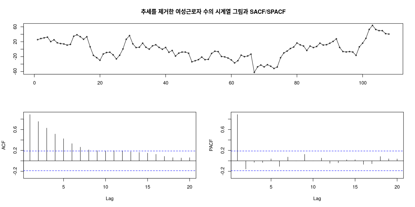
- 0을 중심으로 대칭인것처럼 보이지만.. 확률적 추세가 있어 보이기도 한다..
##H0 : rho1 = ... = rho6 = 0
Box.test(et, lag=6, type = "Ljung-Box")
##H0 : rho1 = ... = rho12 = 0
Box.test(et, lag=12, type = "Ljung-Box")
Box-Ljung test
data: et
X-squared = 259.33, df = 6, p-value < 2.2e-16
Box-Ljung test
data: et
X-squared = 291.08, df = 12, p-value < 2.2e-16- pvalur가 작으니까 오차항이 WN은 아니다.
#H0 : phi=1
fUnitRoots::adfTest(et, lags = 0, type = "nc")
fUnitRoots::adfTest(et, lags = 1, type = "nc")
fUnitRoots::adfTest(et, lags = 2, type = "nc")
Title:
Augmented Dickey-Fuller Test
Test Results:
PARAMETER:
Lag Order: 0
STATISTIC:
Dickey-Fuller: -2.1707
P VALUE:
0.03095
Description:
Tue Nov 28 23:08:43 2023 by user:
Title:
Augmented Dickey-Fuller Test
Test Results:
PARAMETER:
Lag Order: 1
STATISTIC:
Dickey-Fuller: -2.5412
P VALUE:
0.01241
Description:
Tue Nov 28 23:08:43 2023 by user:
Title:
Augmented Dickey-Fuller Test
Test Results:
PARAMETER:
Lag Order: 2
STATISTIC:
Dickey-Fuller: -2.4091
P VALUE:
0.01793
Description:
Tue Nov 28 23:08:43 2023 by user: - H0기각할 수 있다. 차분이 필요하지 않다.
- \(e_t ∼ AR(1)\)
t.test(et)
One Sample t-test
data: et
t = -1.8089e-15, df = 107, p-value = 1
alternative hypothesis: true mean is not equal to 0
95 percent confidence interval:
-4.906433 4.906433
sample estimates:
mean of x
-4.477064e-15 ###### lm (1차추세 모형)
###### et ~ AR(1)
fit_et <- arima(et, order=c(1,0,0),
include.mean = F) ## et
summary(fit_et)
Call:
arima(x = et, order = c(1, 0, 0), include.mean = F)
Coefficients:
ar1
0.9077
s.e. 0.0402
sigma^2 estimated as 122.3: log likelihood = -413.68, aic = 831.37
Training set error measures:
ME RMSE MAE MPE MAPE MASE ACF1
Training set 0.2034053 11.06091 8.125101 -113.0911 259.426 0.9717878 0.1427947파이:0.9077 <- 절대값이 1보다 작으므로 정상 시계열이라고 생각할 수 있다.
1에 가까운 값이니까. 파이^K으로 감소하니까.. 천천히 감소하는 것처럼 보임(acf그래프에서)
lmtest::coeftest(fit_et)
z test of coefficients:
Estimate Std. Error z value Pr(>|z|)
ar1 0.907703 0.040184 22.588 < 2.2e-16 ***
---
Signif. codes: 0 ‘***’ 0.001 ‘**’ 0.01 ‘*’ 0.05 ‘.’ 0.1 ‘ ’ 1- 유의확률이 작게 나와서 정규분포라 하기는 어렵다.. (이상점 떄문에 꼬리)
- 결정적 추세를 분해법을 사용하여 제거한 후 불규칙 성분에 대해 모형 적합 결과
\(Z_t = β_0 + β_1 ∗ t + e_t : \hat Z_t = 186.35 + 4.07t\)
\(e_t = ϕe_{t−1} + u_t, e_t ∼ AR(1) (μ = 0, \hat ϕ = 0.91)\)
\(u_t ∼ WN(0, σ^2)\)
#hat_zt = hat_Tt + hat_et
hat_zt = fitted(fit) + fitted(fit_et)
ts.plot(z, hat_zt, col=1:2, lty=1:2, lwd=2)
legend("topleft", c("z","hat_z"), col=1:2, lty=1:2, lwd=2)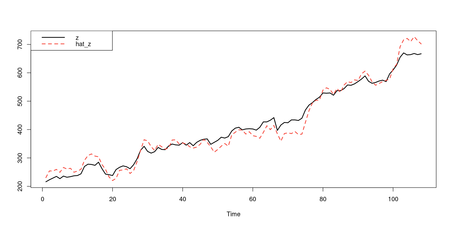
#### ut에 대한 잔차검정
ut <- resid(fit_et)
forecast::tsdisplay(ut)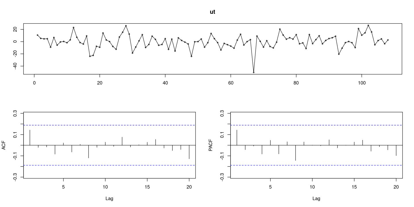
- wn이다
## 정규성검정
tseries::jarque.bera.test(ut) ##JB test H0: normal
Jarque Bera Test
data: ut
X-squared = 56.855, df = 2, p-value = 4.509e-13- 정규분포 아니다. (오차 작은거 하나 있어서)
par(mfrow=c(1,2))
hist(ut)
qqnorm(ut, pch=16)
qqline(ut)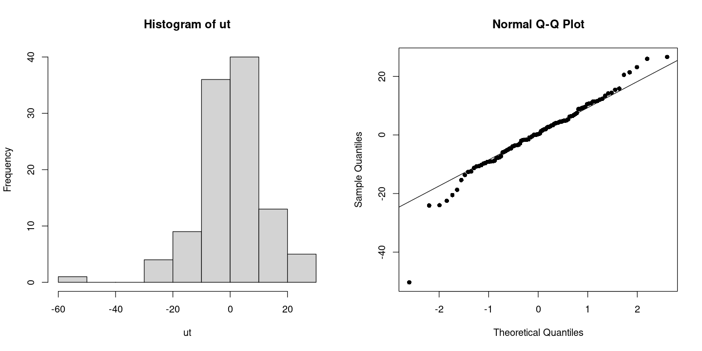
# 잔차의 포트맨토 검정 ## H0 : rho1=...=rho_k=0
portes::LjungBox(fit_et, lags=c(6,12,18,24))| lags | statistic | df | p-value | |
|---|---|---|---|---|
| 6 | 3.677312 | 5 | 0.5967438 | |
| 12 | 6.277097 | 11 | 0.8542505 | |
| 18 | 7.217262 | 17 | 0.9805570 | |
| 24 | 13.987201 | 23 | 0.9272372 |
- 모든 차수에서 rho=0이다. WN이다.
## 잔차 검정
astsa::sarima(et, p=1, d=0, q=0)initial value 3.242671
iter 2 value 2.404146
iter 3 value 2.403718
iter 4 value 2.403704
iter 5 value 2.403697
iter 6 value 2.403671
iter 7 value 2.403663
iter 8 value 2.403662
iter 9 value 2.403646
iter 10 value 2.403646
iter 10 value 2.403646
iter 10 value 2.403646
final value 2.403646
converged
initial value 2.411035
iter 2 value 2.410970
iter 3 value 2.410428
iter 4 value 2.410411
iter 5 value 2.410401
iter 6 value 2.410390
iter 7 value 2.410390
iter 8 value 2.410389
iter 8 value 2.410389
iter 8 value 2.410389
final value 2.410389
converged$fit
Call:
arima(x = xdata, order = c(p, d, q), seasonal = list(order = c(P, D, Q), period = S),
xreg = xmean, include.mean = FALSE, transform.pars = trans, fixed = fixed,
optim.control = list(trace = trc, REPORT = 1, reltol = tol))
Coefficients:
ar1 xmean
0.9078 5.0964
s.e. 0.0400 10.8053
sigma^2 estimated as 122.1: log likelihood = -413.57, aic = 833.13
$degrees_of_freedom
[1] 106
$ttable
Estimate SE t.value p.value
ar1 0.9078 0.0400 22.6947 0.0000
xmean 5.0964 10.8053 0.4717 0.6381
$AIC
[1] 7.714211
$AICc
[1] 7.71527
$BIC
[1] 7.788715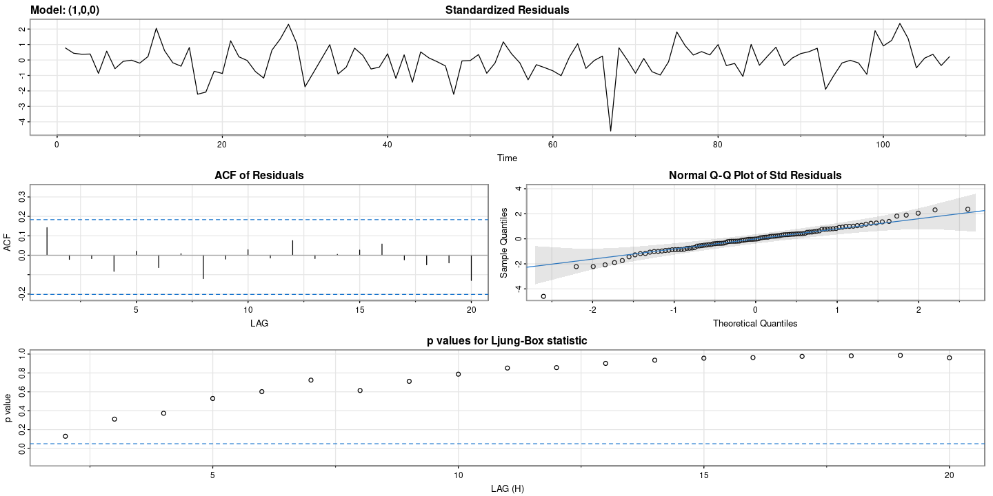
결정적 추세가 아니라 확률적 추세라고 생각하고 차분을 진행하여 추세 성분 제거한 후 적합하기
## 차분
diff_z = diff(z)
forecast::tsdisplay(diff_z)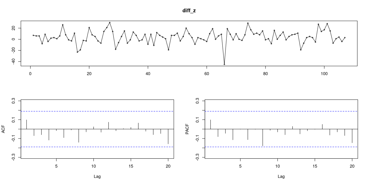
- 차분한 데이터가 WN이다.
Box.test(diff(z), lag=6, type = "Ljung-Box")
Box.test(diff(z), lag=12, type = "Ljung-Box")
Box-Ljung test
data: diff(z)
X-squared = 4.5688, df = 6, p-value = 0.6002
Box-Ljung test
data: diff(z)
X-squared = 7.895, df = 12, p-value = 0.7933t.test(diff(z))
One Sample t-test
data: diff(z)
t = 3.8382, df = 106, p-value = 0.0002111
alternative hypothesis: true mean is not equal to 0
95 percent confidence interval:
2.037736 6.392171
sample estimates:
mean of x
4.214953 - 0은 좀 아닌거 같다..?
# Zt ~ radomwalk, ARIMA(0,1,0) with drift
## 모형 ARIMA(0,1,0)
fit <- arima(z,order=c(0,1,0))
summary(fit)
Call:
arima(x = z, order = c(0, 1, 0))
sigma^2 estimated as 145.6: log likelihood = -418.3, aic = 838.6
Training set error measures:
ME RMSE MAE MPE MAPE MASE ACF1
Training set 4.177926 12.01043 9.085333 0.990671 2.414276 0.9909589 0.09736789\(Z_t = Z_{t−1} + ε_t\): random walk
\(Z_t = δ + Z_{t−1} + ε_t\): random walk with drift
\((1 − B)Z_t = δ + ϵ_t\) : 모형에 차분한 데이터를 넣어줌.
fit2 <- arima(diff_z, order=c(0,0,0)) #알아서 mean을 적합해줌
summary(fit2)
Call:
arima(x = diff_z, order = c(0, 0, 0))
Coefficients:
intercept
4.215
s.e. 1.093
sigma^2 estimated as 127.8: log likelihood = -411.34, aic = 826.68
Training set error measures:
ME RMSE MAE MPE MAPE MASE ACF1
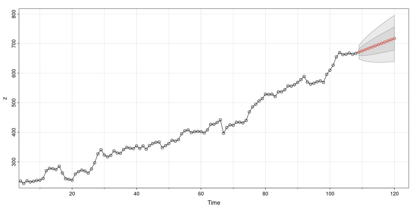
Training set 2.091723e-15 11.30629 8.354441 -Inf Inf 0.7330884 0.09829173- 차분을 이용하여 적합한 최종 모형
\(Z_t = δ + Z_{t−1} + ε_t\): random walk with drift
\(ε_t ∼ WN(0, σ^2)\)
\(\hat δ = 4.215, \hat σ^2 = 127.8\)
- AIC가 더 작아졌다. drift가 있는 모형이 더 좋다
### 잔차검정
resid = resid(fit2)
forecast::tsdisplay(resid)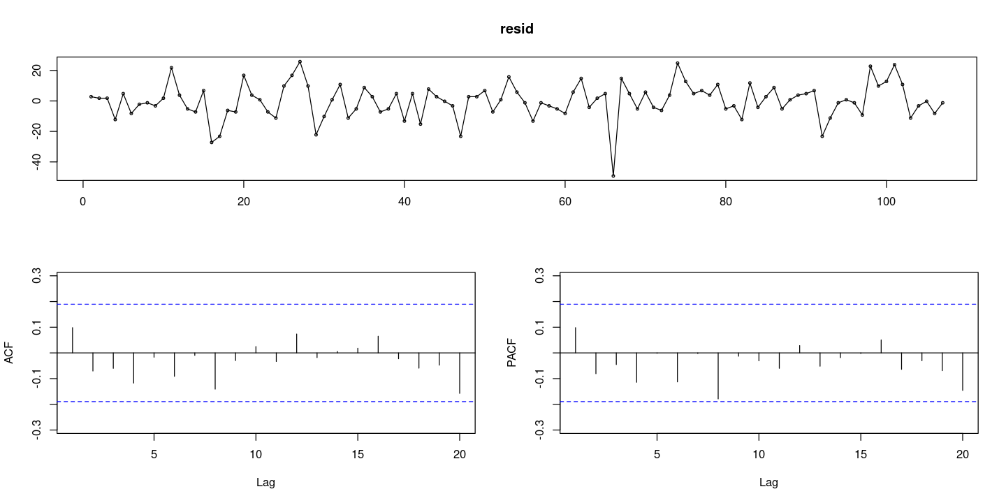
## 정규성검정
tseries::jarque.bera.test(resid) ##JB test H0: normal
Jarque Bera Test
data: resid
X-squared = 40.633, df = 2, p-value = 1.502e-09par(mfrow=c(1,2))
hist(resid)
qqnorm(resid)
qqline(resid)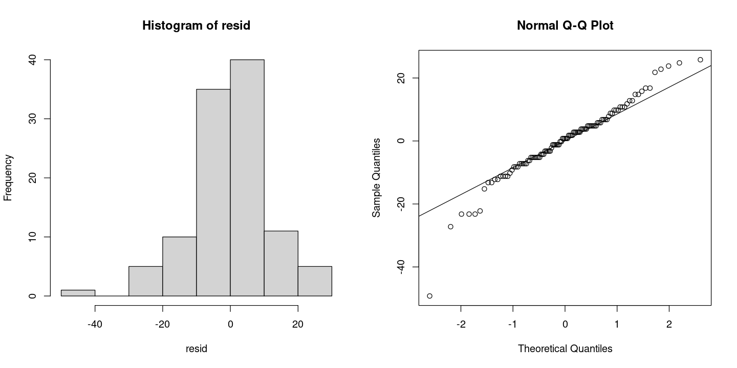
# 잔차의 포트맨토 검정 ## H0 : rho1=...=rho_k=0
portes::LjungBox(fit_et, lags=c(6,12,18,24))| lags | statistic | df | p-value | |
|---|---|---|---|---|
| 6 | 3.677312 | 5 | 0.5967438 | |
| 12 | 6.277097 | 11 | 0.8542505 | |
| 18 | 7.217262 | 17 | 0.9805570 | |
| 24 | 13.987201 | 23 | 0.9272372 |
## 잔차 검정
astsa::sarima(z, p=0, d=1, q=0)
initial value 2.425360
iter 1 value 2.425360
final value 2.425360
converged
initial value 2.425360
iter 1 value 2.425360
final value 2.425360
converged$fit
Call:
arima(x = xdata, order = c(p, d, q), seasonal = list(order = c(P, D, Q), period = S),
xreg = constant, transform.pars = trans, fixed = fixed, optim.control = list(trace = trc,
REPORT = 1, reltol = tol))
Coefficients:
constant
4.215
s.e. 1.093
sigma^2 estimated as 127.8: log likelihood = -411.34, aic = 826.68
$degrees_of_freedom
[1] 106
$ttable
Estimate SE t.value p.value
constant 4.215 1.093 3.8562 2e-04
$AIC
[1] 7.725979
$AICc
[1] 7.726336
$BIC
[1] 7.775939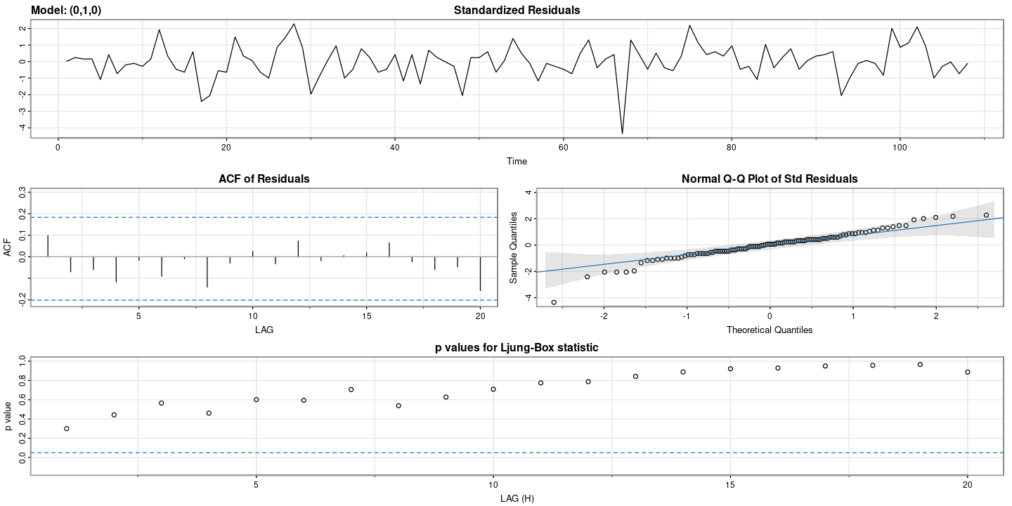
astsa::sarima.for(z, n.ahead=12, p=0, d=1, q=0)- $pred
- A Time Series:
- 671.21495327103
- 675.429906542061
- 679.644859813091
- 683.859813084122
- 688.074766355152
- 692.289719626183
- 696.504672897213
- 700.719626168244
- 704.934579439274
- 709.149532710305
- 713.364485981335
- 717.579439252366
- $se
- A Time Series:
- 11.306294696503
- 15.9895152999816
- 19.5830768596898
- 22.612589393006
- 25.2816435150261
- 27.694652887968
- 29.9136440165555
- 31.9790305999631
- 33.918884089509
- 35.7536431380317
- 37.4987372774857
- 39.1661537193795